The Main Principles Of Vlookup For Dummies

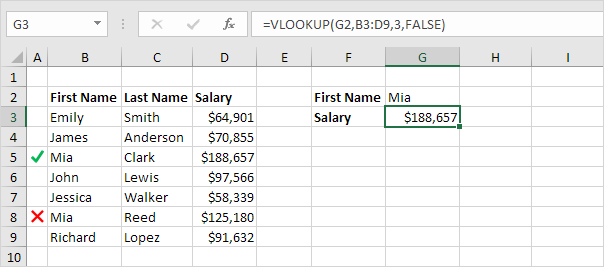
Use VLOOKUP when you require to find points in a table or a range by row. For example, search for a price of an automotive component by the part number, or find a staff member name based on their worker ID. In its simplest kind, the VLOOKUP feature says: =VLOOKUP(What you intend to look up, where you intend to try to find it, the column number in the variety including the value to return, return an Approximate or Specific match-- suggested as 1/TRUE, or 0/FALSE).

Make use of the VLOOKUP function to search for a worth in a table. Phrase structure VLOOKUP (lookup_value, table_array, col_index_num, [range_lookup] For instance: =VLOOKUP(A 2, A 10: C 20,2, TRUE) =VLOOKUP("Fontana", B 2: E 7,2, FALSE) =VLOOKUP(A 2,'Client Information'! A: F,3, FALSE) Disagreement name Summary lookup_value (required) The worth you want to seek out. The worth you wish to search for need to be in the very first column of the variety of cells you define in the table_array argument.

Lookup_value can be a value or a recommendation to a cell. table_array (required) The variety of cells in which the VLOOKUP will look for the lookup_value and the return value. You can make use of a named array or a table, and you can make use of names in the disagreement rather of cell recommendations.

The cell range also needs to consist of the return worth you wish to find. Find out exactly how to select arrays in a worksheet. col_index_num (required) The column number (starting with 1 for the left-most column of table_array) that contains the return worth. range_lookup (optional) A rational worth that specifies whether you want VLOOKUP to locate an approximate or an exact suit: Approximate match - 1/TRUE presumes the initial column in the table is sorted either numerically or alphabetically, and also will after that look for the closest value.

For instance, =VLOOKUP(90, A 1: B 100,2, TRUE). Exact suit - 0/FALSE look for the exact worth in the first column. As an example, =VLOOKUP("Smith", A 1: B 100,2, FALSE). There are 4 pieces of info that you will certainly need in order to build the VLOOKUP syntax: The worth you want to seek out, likewise called the lookup value.

Rumored Buzz on How To Do A Vlookup

Keep in mind that the lookup value need to constantly be in the first column in the variety for VLOOKUP to work correctly. For instance, if your lookup worth is in cell C 2 then your range need to start with C. The column number in the array which contains the return value. For instance, if you specify B 2:D 11 as the range, you must count B as the initial column, C as the 2nd, and so forth.

If you don't define anything, the default value will certainly constantly hold true or approximate match. Currently put all of the above together as adheres to: =VLOOKUP(lookup worth, range consisting of the lookup value, the column number in the array including the return value, Approximate match (REAL) or Exact match (FALSE)). Here are a few instances of VLOOKUP: Issue What failed Incorrect worth returned If range_lookup is TRUE or overlooked, the very first column needs to be arranged alphabetically or numerically.

Either kind the very first column, or make use of FALSE for a specific suit. #N/ A in cell If range_lookup is REAL, after that if the worth in the lookup_value is smaller sized than the smallest worth in the very first column of the table_array, you'll obtain the #N/ An error worth. If range_lookup is FALSE, the #N/ A mistake worth indicates that the specific number isn't found.

#REF! in cell If col_index_num is better than the variety of columns in table-array, you'll obtain the #REF! error worth. For more details on fixing #REF! mistakes in VLOOKUP, see Exactly how to correct a #REF! error. #VALUE! in cell If the table_array is much less than 1, you'll get the #VALUE! mistake worth.

#NAME? in cell The #NAME? mistake value typically indicates that the formula is missing quotes. To seek out a person's name, make certain you make use of quotes around the name in the formula. For instance, enter the name as "Fontana" in =VLOOKUP("Fontana", B 2: E 7,2, FALSE). For more details, see Just how to fix a #NAME! error.

Some Known Facts About How To Vlookup.

Discover exactly how to utilize outright cell recommendations. Do not save number or date worths as text. When looking number or date values, make certain the information in the very first column of table_array isn't stored as message values. Or else, VLOOKUP might return a wrong or unforeseen value. Arrange the very first column Kind the very first column of the table_array prior to utilizing VLOOKUP when range_lookup holds true.

A concern mark matches any kind of solitary personality. An asterisk matches any type of series of characters. If you intend to discover an actual enigma or asterisk, kind a tilde (~) before the character. For example, =VLOOKUP("Fontan?", B 2: E 7,2, FALSE) will look for all instances of Fontana with a last letter that might vary.

When browsing text worths in the first column, see to it the information in the very first column does not have leading spaces, routing areas, inconsistent use straight (' or") as well as curly (' or ") quotation marks, or nonprinting characters. In these situations, VLOOKUP could return an unexpected value.

You can always ask a specialist in the Excel Individual Voice. Quick Recommendation Card: VLOOKUP refresher Quick Reference Card: VLOOKUP troubleshooting suggestions You Tube: VLOOKUP video clips from Excel community experts Everything you require to find out about VLOOKUP Just how to deal with a #VALUE! mistake in the VLOOKUP function Exactly how to deal with a #N/ An error in the VLOOKUP function Overview of formulas in Excel Exactly how to stay clear of damaged solutions Find mistakes in solutions Excel features (indexed) Excel functions (by group) VLOOKUP (totally free sneak peek).

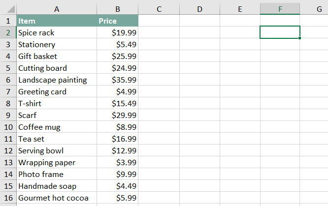
To calculate shipping cost based upon weight, you can make use of the VLOOKUP feature. In the example revealed, the formula in F 8 is: =VLOOKUP(F 7, B 6: C 10,2,1)* F 7 This formula uses the weight to find the proper "expense per kg" then ... To override output from VLOOKUP, you can nest VLOOKUP in the IF function.

vlookup formula in excel hindi excel vlookup in pivot excel vlookup increase column index number